Learning Data Science, Day 3 – Mathematical Functions
Okay, back to the data science. This is all under a heading titled "DS Math", which kinda terrifies me, not going to lie, because even though I know data science needs mathematics, it's not my strongest subject, and numbers have a tendency to get really wonky on me.
Like, I will transpose digits at the drop of a hat. Phone numbers are a regular issue for me, especially if someone's reading them aloud to me. I once wrote "23" in a recipe instead of "2-3" and ended up with 23 tablespoons of water in an icing.
Numbers and I? We are not friends. But I can get through this, yes I can.
Linear Functions
So a function relates one variable to another. Okay. And a linear function has an independent variable and a dependent variable.
They use calories and pulse as an example, but I also dislike that example, because it correlates caloric loss with raised pulse, and, okay, yeah, that is a way to burn calories, but ugggh I just hate calorie counting in general, it reminds me too much of all the Weight Watcher and dieting rigamarole of my childhood, all skim milk and brown bread.
So, instead, I'm going to come up with a new example.
The independent variable is the number of bookcases in a house. The dependent variable in the number of books. You need the bookcases to store the books, so if you know the number of bookcases, you can figure out the number of books.
(Yes, this is assuming that all the books and all the bookcases are the same size, and you're not like me and sticking random things like Funko Pops and Minas Tirith statues and Lightcycles on the bookshelves as well. Just go with it.)
They then say that linear functions have a specific form:
y = f(x) = ax + b
This calculates the value for the dependent variable once we choose a value for the independent variable.
In this function, all the bits are:
f(x): the output (the dependent variable)x: the input (the independent variable)a: slope, which is the coefficient of the independent variable and gives the rate of change of the dependent variableb: intercept, which is the value of the dependent variable whenx = 0, and is also the point where the diagonal line crosses the vertical axis
No, slope and intercept don't quite make sense to me yet. But I'll get there.
Linear Functions with One Explanatory Variable
So then they change it up, and say that they have a linear function with a variable that's used for prediction.
Which would be if we wanted to predict how many books we could buy at one of those "£10 for a bag full of books" sales, we'd count the number of empty bookcases we have, and have a fixed value as well (the number of books we already have)
The formula here is:
f(x) = 50x + 200
And the bits are:
f(x): The output, where we get the predicted number of booksx: The input, which are the bookshelves50: The slope, specifying how many books fill up a bookcase200: The intercept, specifying how many books we have in the house when we have no empty bookshelves
Plotting a Linear Function
When you show a linear function in a graph, it'll always be a straight line — hence, linear. So if I were to graph out the function above:
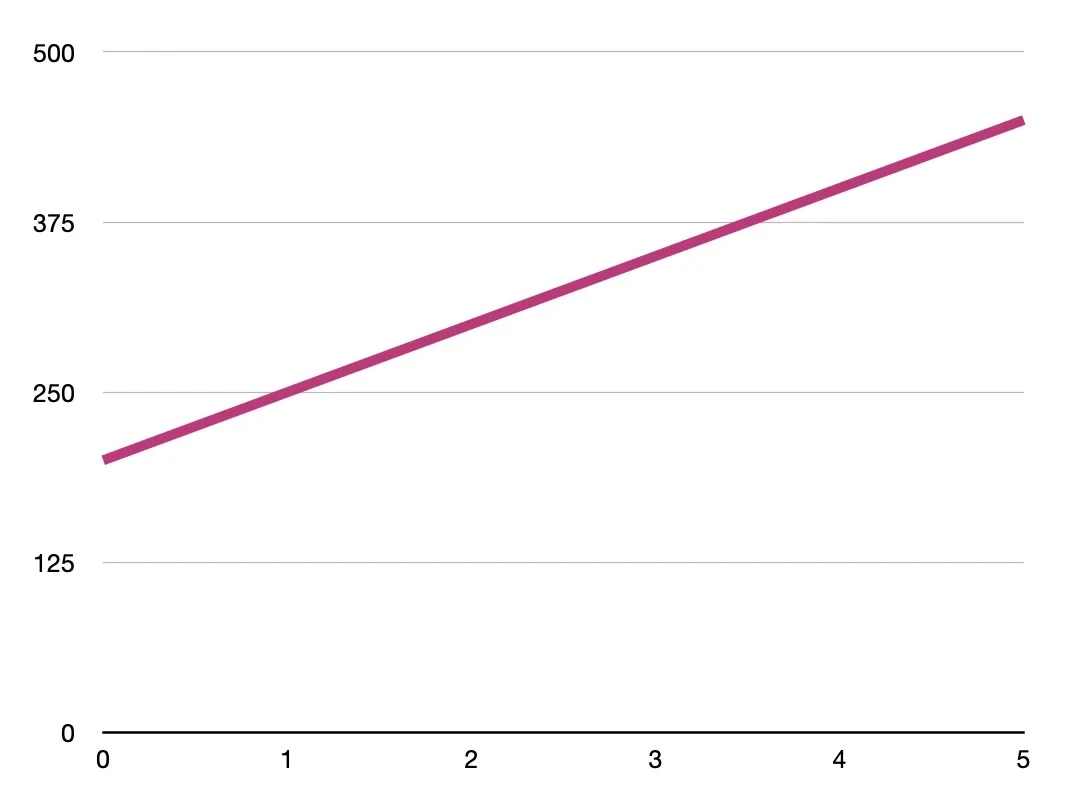
I already have 200 books. For each empty shelf I have, I can purchase another 50 books. If I had five empty shelves, I could buy 250 more books. If I only had two empty shelves, I could only buy 100 more books. And if all my shelves are already full, well, I have 200 books I probably haven't read yet.
So that's how a linear function works.
Plotting Existing Data Into Python
Now we need to put it into Python.
So we have the table
| Shelves | Books |
|---|---|
| 0 | 200 |
| 1 | 250 |
| 2 | 300 |
| 3 | 350 |
| 4 | 400 |
| 5 | 450 |
Or, as our CSV would be:
Shelves,Books
0,200
1,250
2,300
3,350
4,400
5,450
So first, we have to import in some libraries to make the W3Schools compiler draw the graph. I don't know if I'd have to do this with another compiler, but, hey, it's good to have in place.
import sys
import matplotlib
matplotlib.use('Agg')
Then we have to import Pandas to read the CSV and MatPlotLIb to plot the data.
import pandas as pd
import matplotlib.pyplot as plt
Then we'd read the CSV.
books_data = pd.read_csv("data.csv", header = 0, sep = ",")
Then we'd use plot() to plot the points.
books_data.plot(x = 'Shelves', y = 'Books', kind ='line'),
plt.ylim(ymin = 0)
plt.xlim(xmin = 0)
kind='line' says what kind of plotting we want — it wants to be a straight line. And ylim() and xlim() say what value we want the axes to start on. Since we want both on zero, we have ymin = 0 and xmin = 0.
(ymax and xmax do the same, but for the maximum amounts we want to show on the graph.)
Then we show the output
plt.show()
There are two more lines to make the W3Schools compiler be able to draw, so I'm including these in as well.
plt.savefig(sys.stdout.buffer)
sys.stdout.flush()
So then I hit "Run", and I get
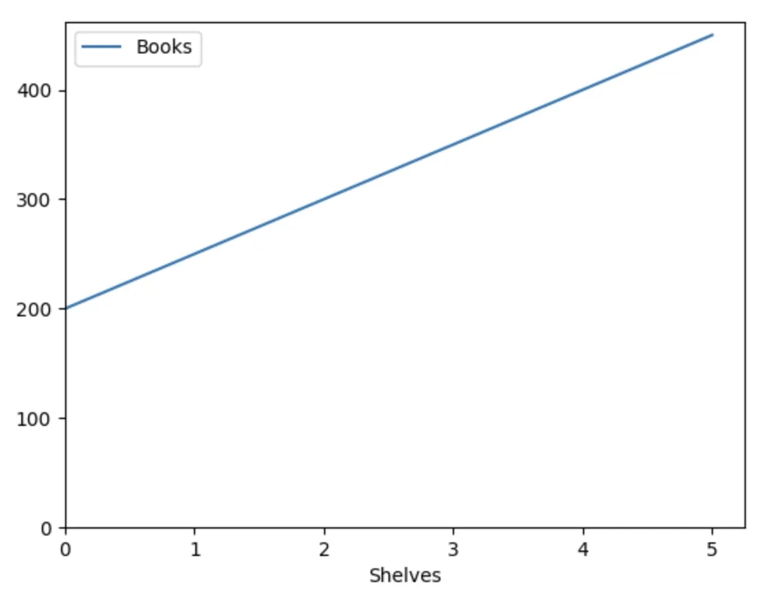
Neat.
But what if I didn't count the already full shelves?
Let's drop 0 from our CSV and rerun it.
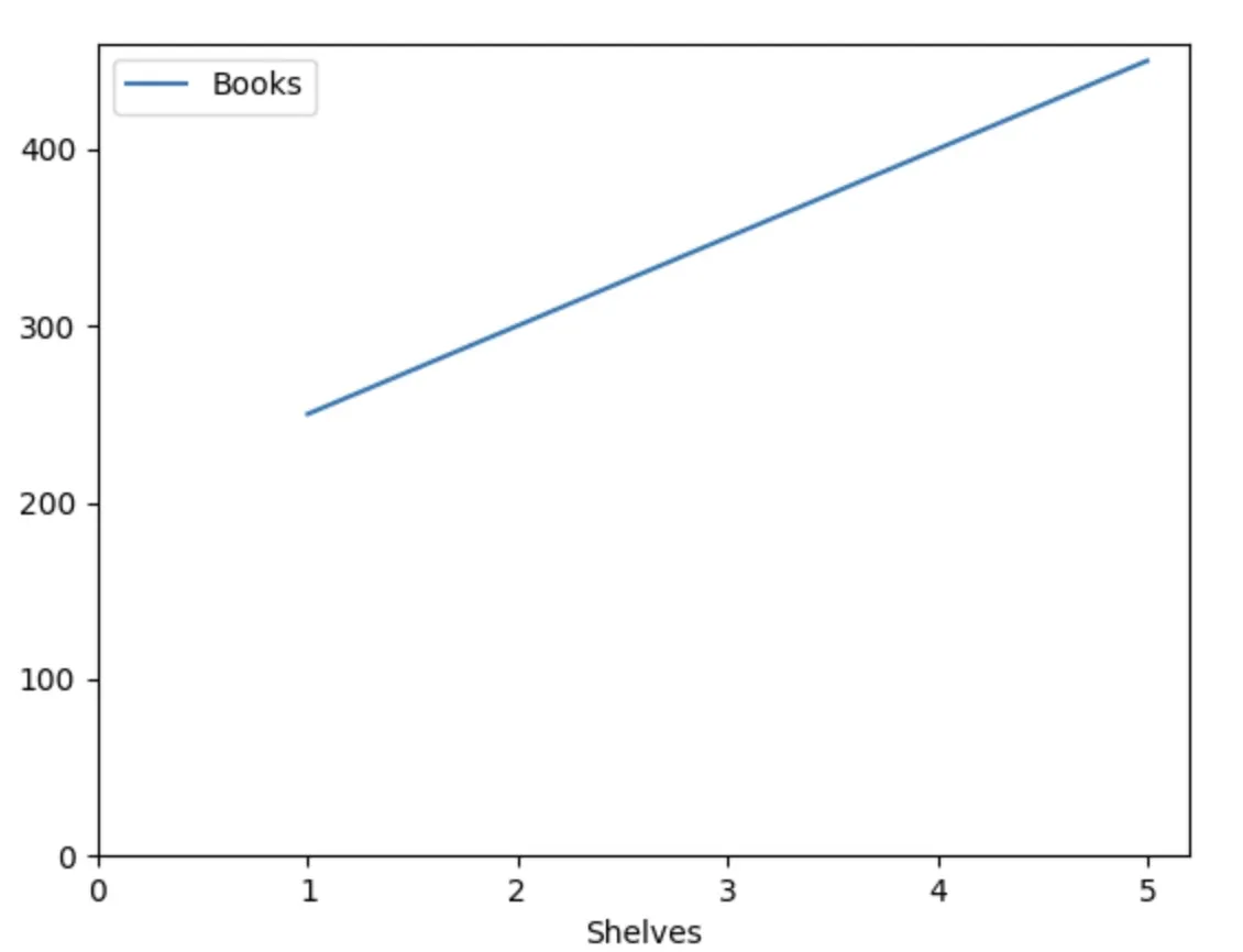
Now it starts in the middle, because there's no 0 column, but it's still linearly progressing, 50 more books for every shelf.
Determining Slope
But what if I didn't know that it was 50 books per shelf or that I already had 200 books? What if I just had a huge pile of books and I had to shelve them?
That's where I figure out the slope and intercept from the graph.
So we take our second graph, the one where we don't have the 0 shelf, and use the proportional difference between two points.
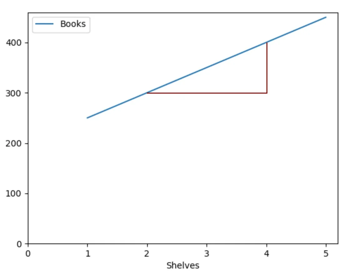
Since we can see that 2 Shelves = 300 Books, and 4 Shelves = 400 books, we can figure out the slope by doing the proportions.
They have a formula for it too.
Slope = f(x2) - f(x1) / x2-x1
So with our data, f(x2) is 400, f(x1) is 300, x2 is 4, and x1 is 2. Pop that into the equation...
Slope = (400 - 300) / (4 - 2) = 50
And there's our slope.
You can also use Python to find the slope, which does the exact same formula, just written in Python so it does the subtraction and division for you.
def slope(x1, y1, x2, y2):
  s = (y2-y1)/(x2-x1)
  return s

print(slope(2,300,4,400))
And there you go, another 50.
Determining Intercept
So, obviously, we already have books, but how many do we already have?
We could just draw a straight line using the graph...
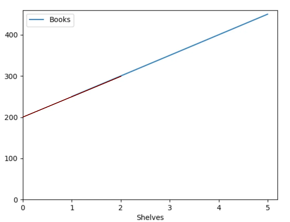
Or, because we know the slope is 50 and two shelves mean 300 books, we could just keep subtracting 50 until we reached 0.
2   - 1  = 1
300 - 50 = 250
1   - 1  = 0
250 - 50 = 200
But this is data science and we're gonna have more complicated numbers most of the time. So it's time to get Python to get the slope and intercept.
First we import Pandas and NumPy to read the CSV and do the maths.
import pandas as pd
import numpy as np
Then we read the CSV.
books_data = pd.read_csv("data.csv", header = 0, sep = ",")
Then we tell the program what x and y are.
x = books_data["Shelves"]
y = books_data["Books"]
Then NumPy tells us the slope and intercept.
slope_intercept = np.polyfit(x,y,1)
print(slope_intercept)
When a function is linear, you put 1 into the polyfit(), because everything is in the power of one.
When we run that program, we get
[ 50. 200.]
Which is the slope (50) and the intercept (200).
We can now predict the number of books we can get by using the expression
f(x) = 50x + 200
Which means that if we've turned a whole room into nothing but shelves, and have 80 shelves at our disposal...
f(80) = (50 * 80) + 200
Or, to put it in Python terms
def books(x):
  return 50*x + 200
print (books(80))
Yep, I'm buying 4,200 more books.
Day 3 — Results
- Functions relate variables to each other.
- Linear functions have an independent variable and a dependent variable. Or you can write it as
y = f(x) = ax + b. - Slope is the coefficient of the independent variable and gives the rate of change of the dependent variable.
- Intercept is the value of the dependent variable when your independent variable is 0.
- So it's
Dependent = (Slope * Independent) + Intercept. - You can use MatPlotLib to plot your linear functions.
plot()plots the points. You use it likeDATA_SET.plot(x = 'DATA_X', y = 'DATA_Y', kind = 'line').- If you add
ylimandxlimto your code as well, you can limit the axes in your graph.xminandymindo the minimum,xmaxandymaxdo the maximum. - You ask MatPlotLib to show you the graph by using
.show() - You can use NumPy to determine the slope and intercept of your data. Use
.polyfit(x,y,1).
That wasn't anywhere near as terrible as I thought it'd be, and now I know how to make linear graphs in Python, which is nice.
We'll get into statistics after this, which will be...something. I'm not sure yet.
Today's Sticker

Who's that Pokémon? It's Farfetch'd!
Did you see the trailer for The Misadventures of Sirfetch'd & Pichu? Okay, it's not as tooth-rottingly adorable as Pokémon Concierge, but it is still ridiculously cute and will be a delight to watch.