Learning Data Science, Day 7 - Linear Regression
I'm not going to lie, I'm a bit sleepy and prone to just wanting to doze and listen to all the audiobooks of Lois McMaster Bujold's Vorkosigan saga (I'm in the middle of a relisten of Memory at the moment), but, no, I told myself I was going to do work today, so we're back onto the data science.
W3Schools has labeled this section "Data Science Advanced", so, y'know, oooo, fancy. We're getting advanced here.
Linear Regression
So "regression" when you're referring to data science, isn't when you take a bunch of hallucinogens and lie in a sensory deprivation tank and get all Altered States up in here, it's when you try to find the relationship between your variables.
When you do statistical modelling, you use regression to predict the outcome of things. In their example, because it's all still health data, it's working out if average pulse and duration of exercise are related to calories burned, but...borrrrrring. So BORING.
I'm going back to my Letterboxd decades, watched films, and films I loved data. Because then I can work out if the decade and the number of films I watched are related to the films I love. Yeah. That'll work, right?
It does mean I have to tweak the data a bit, though.
| Decade | Watched | Liked |
|---|---|---|
| 1910 | 3 | 0 |
| 1920 | 4 | 0 |
| 1930 | 16 | 0 |
| 1940 | 56 | 3 |
| 1950 | 123 | 3 |
| 1960 | 142 | 6 |
| 1970 | 132 | 5 |
| 1980 | 116 | 17 |
| 1990 | 34 | 11 |
| 2000 | 26 | 3 |
| 2010 | 189 | 12 |
| 2020 | 174 | 10 |
(I know this means it'll try and give me an average of the year or whatever, but, eh, I'll see how it goes.)
Least Square Method
Linear regression, when the relationship between the variables is a straight line, uses the least square method. You plot all the points on a graph, and then you try to draw a straight line that has a minimal distance to all the data points.
The distance from the line to the plotted point is called a "residual" or an "error". You want that to be as close to 0 as possible.
So let's take my film data, and see what linear regression we get when we talk about how many films from each decade I watched.
We're going to use Pandas, MatPlotLib, and SciPy, so we have to import those in first.
import pandas as pd
import matplotlib.pyplot as plt
from scipy import stats
Then we get Pandas to read the CSV and tell it what X and Y are going to be.
film_data = pd.read_csv("data.csv", header=0, sep=",")

x = film_data["Decade"]
y = film_data["Watched"]
Then we use SciPy to do .linregress(x,y) on the data, which will give us the slope, the intercept, r, p, and the standard error. (I'm not 100% certain what r and p are. I'll have to look that up.)
slope, intercept, r, p, std_err = stats.linregress(x, y)
Create a new function that does some maths on the slop and the intercept.
def myfunc(x):
 return slope * x + intercept
Create a new array that lists all the points created with that function.
mymodel = list(map(myfunc, x))
And then plot out your data as a scatter plot, and use your fancy new array to create the linear regression line that matches up to your plot points. Tweak the x and y limitations as needed.
plt.scatter(x, y)
plt.plot(x, mymodel)
plt.ylim(ymin=0, ymax=200)
plt.xlim(xmin=1900, xmax=2030)
plt.xlabel("Decade")
plt.ylabel ("Watched")
plt.show()
And there you go. A nice straight line that vaguely matches up.
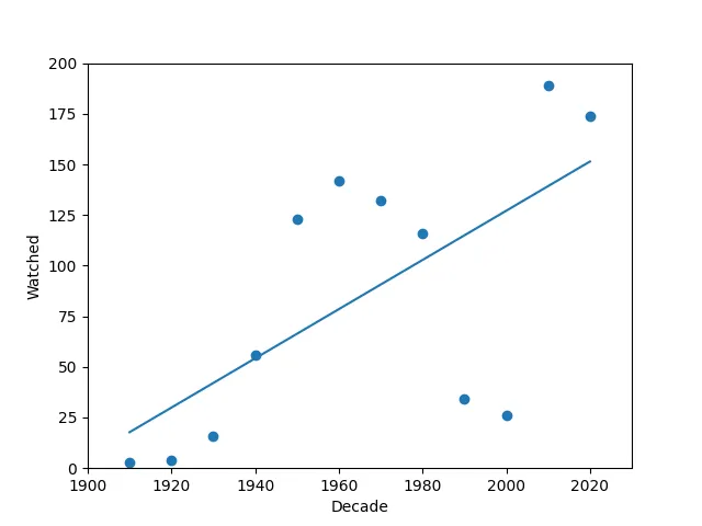
It obviously doesn't match up well, though. I mean, the only one it actually goes through is the 1940s, and it kinda gets near the 1980s, but then it's way off with the 1990s and 2000s.
So it's not the best predictor of what decades I'm going to watch. I mean, okay, the more recent the film, the more likely it is that I watch it, because, yeah, I watch new movies, but it's...kinda lacking.
Regression Table
You can get more detail about your linear regression output by creating a regression table. That's a nice little table that gives you a bunch of details about your data, including:
- Information about the model
- Coefficients of the linear regression function
- Regression statistics
- Statistics of the coefficients from the linear regression function
This is going to give you a heck of a lot of data, most of which you need more than a basic online data science course to understand. You need, like, a proper statistics course. I should really take one.
And the example doesn't let you try it out, so I can't even try to figure it out using my data. It involves the statsmodels.formula.api library, so I guess that might be too big or too expensive for dweebs like me to try out.
But here's the code they use and the table they get back. It's the health data again.
import pandas as pd
import statsmodels.formula.api as smf

full_health_data = pd.read_csv("data.csv", header=0, sep=",")

model = smf.ols('Calorie_Burnage ~ Average_Pulse', data = full_health_data)
results = model.fit()
print(results.summary())
.ols() creates the model based on the Ordinary Least Squares. And then once you have that model, you run that data through .fit(), which gives you the variable results. Then it's just .summary() to get this pretty table. (I'm using a screenshot instead of copy/pasting the actual plain text, because...it's a lot.)
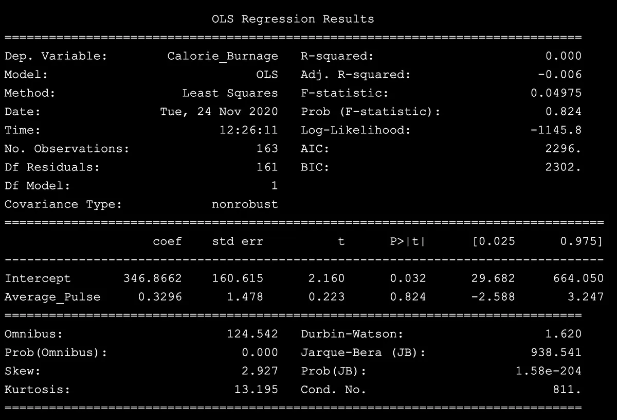
That's a lot of data. And so much of it is beyond me, especially since I can't put in my own data.
But W3Schools goes through a bunch of the bits in this table.
Up at the top, where it says Dep. Variable:, Model:, Method:, Date:, Time:, and No. Observations, that's the Information section. It tells you what the dependent variable is, what type of model was used (Ordinary Least Squares or OLS), the method used, the date and time, and the number of observations in the data (the number of entries).
They then focus on the coefficient, which is the output of your linear regression function.
The linear regression function can be written mathematically as:
Your Dependent Variable =
Your Independent Variable's Coefficient *
Your Independent Variable +
Intercept Point
So once you know your Independent Variable's Coefficient and your Intercept Point, you can start to predict what your Dependent Variable will be depending on your Independent Variable.
They do an example in Python, but since it's just maths, it's not that exciting. I need to be able to put in my own data and get my own results for me to care about plugging in the numbers.
And because I still can't plug in my own data, I'm going to leave the last three parts of this Data Science module until Wednesday. Maybe I'll be able to find a place where I can put in .ols() into something without having to pay more.
Day 7 — Results
- Regression is the relationship between your variables.
- Linear regression is the straight line you can draw that is as close as possible to the plotted points in your graph.
- This uses the least square method.
- The distance from the line to your plotted point is called the residual or the error.
- You use SciPy to do the linear regression on your data, using
.linregress(x,y) - It'll return the slope, the intercept, the r, the p, and the standard error.
- You can then define a function based on the slope, the intercept, and your X data.
- Which plots onto your Y axis and gives you the nice line between all your data.
- You can also get a lot of information about your data by building a Regression Table.
- This uses the
statsmodels.formula.apilibrary, using.ols()to create the model,.fit(), to get the variables, and.summary()to get the table. - The linear regression function can be written as
Y = Coefficient of X * X + Intercept
Today's Sticker
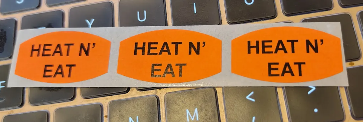
Shifty Sticker Club strikes again!
Heat n' Eat! Heat n' Eat! Heat n' Eat!
Someone should turn this into a SVG and get it printed on a pair of booty shorts. Hell yeah.