Learning Data Science, Day 8 - Linear Regression, with actual data
After a busy day running errands and seeing films, I'm back to finish off the Data Science course.
So, last time, we had the regression table that we couldn't generate, but we did have a nice little regression chart. Let's see what we'll be able to do today.
Linear Regression Table
I was going to keep using the data they showed, and complain about how I couldn't get my own data working...and I realised I can just set up Python on this Mac.
...
I'm not the smartest person sometimes.
So we're going back to the beginning of the regression table, so I can work out what it all means while also using my film data.
We are, however, tweaking my film data again, because Decades is going to throw us off. Instead, I'm going to take all the films I've watched between 2018 and 2025, count them by those years, and also count how many of them are in the "Films I Like" count as well.
| Year | Watched | Liked |
|---|---|---|
| 2018 | 73 | 1 |
| 2019 | 166 | 3 |
| 2020 | 70 | 2 |
| 2021 | 98 | 16 |
| 2022 | 129 | 18 |
| 2023 | 126 | 25 |
| 2024 | 93 | 11 |
| 2025 | 156 | 20 |
I cleared out films that I saw multiple times within the same year, but left them in if I watched them again in a different year. So, yeah, Dune (1984) does get counted four times, but that's because I watched it four years in a row. We don't talk about how many times I watched it during those four years, but...
Yeah.
So. We will try to predict "Films I Like" with "Films I've Watched" using Linear Regression.
First, we do the linear regression graph. This one, we do in the W3Schools engine, because we can.
import pandas as pd
import matplotlib.pyplot as plt
from scipy import stats

film_data = pd.read_csv("data.csv", header=0, sep=",")

x = film_data["Watched"]
y = film_data["Liked"]

slope, intercept, r, p, std_err = stats.linregress(x, y)

def myfunc(x):
 return slope * x + intercept

mymodel = list(map(myfunc, x))

plt.scatter(x, y)
plt.plot(x, mymodel)
plt.ylim(ymin=0, ymax=25)
plt.xlim(xmin=50, xmax=170)
plt.xlabel("Watched")
plt.ylabel ("Liked")
plt.show()
I had to do some tweaking with the xlim and ylim to make it a little more visible, but we have a plotted linear regression.
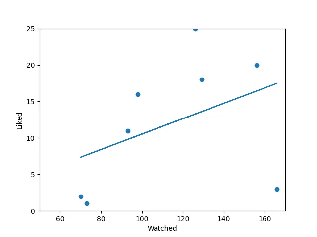
The plotted points are a little scattershot, but it still shows that the more movies I see, the more likely it is that I've watched movies I like.
(I mean, I like most of them. I just love some of them.)
Then we set up the Linear Regression Table in Python, using the code W3Schools gives us, but putting it into my terminal rather than in W3Schools.
import pandas as pd
import statsmodels.formula.api as smf

film_data = pd.read_csv("movies.csv", header=0,sep=",")

model = smf.ols('Liked ~ Watched', data = film_data)
results = model.fit()
print(results.summary())
And when we run that...
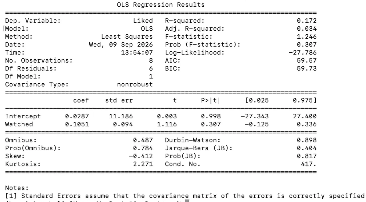
YAY. DATA.
So let's go through all the sections that W3Schools goes through.
Information in the Regression Table
The first section they focus on is the Information section, which is this:
Dep. Variable:		Liked
Model:			OLS
Method:			Least Squares
Date:			Wed, 09 Sep 2026
Time:			13:54:07
No. Observations:	8
- Dep. Variable is the dependent variable, which is assumed to be explained by the explanatory variable (Watched).
- Model is what was used. OLS is Ordinary Least Squares, and uses the Least Square Method.
- Date and Time are, welp, the date and time I ran the script.
Coefficients in the Regression Table
Then we focus on the coefficients, which are under the second === line and are these:
		coef
Intercept	0.0287
Watched		0.1051
The coefficient here for Watched is the output of the linear regression function, which can be rewritten as a formula:
Liked Films = 0.1051 * Watched Films + 0.0287
If the number of Watched Films increases by 1, the number of Liked Films increases by 0.11.
If the number of Watched Films is 0, the number of Liked Films is 0.029.
So then I can define the function in Python to make predictions. Like, if I watch 300 films. Or 20. Or 1000.
def Predict_Likes(Watched):
 return(0.1051 * Watched + 0.0287)

print(Predict_Likes(300))
print(Predict_Likes(20))
print(Predict_Likes(1000))
And I get:
31.5587
2.1307
105.1287
Which is pretty neat to know. Right now, in 2026, according to Letterboxd, I've seen 89 films so far. And based on this formula, out of those 89, 9.3826 will be films I love. When I look at my diary, I loved 7 of the 89 films I've seen this year, so, y'know, it's not too far off.
Statistics of Coefficients and P-value in the Regression Table
So now we look at the rest of the Coefficients data in the table.
		coef	std err	t 	P>|t|	[0.025 	0975]
Intercept	0.0287 	11.186 	0.003 	0.998 	-27.343 27.400
Watched		0.1051 	0.094 	1.116 	0.307 	-0.125 	0.336
This is if we want to test whether or not the coefficients from the linear regression function have an impact on the dependent variable. We want to prove that a relationship between Films Watched and Films Liked exists using statistical tests, and these stats here help us.
std erris the Standard Error.tis the "t-value" of the coefficients.P>|t|is the "P-value".[0.025 0.975]are the confidence value.
First we focus on the "P-value". That's a number to conclude if there's a relationship between the two variables.
There are three results that we can get with the P-value:
- Equal to 0: There's no relationship between the variables.
- Less than 0.05: It's not likely to equal 0, so it's a low P-value.
- More than 0.05: We can't conclude that the explanatory variable affects the dependent variable, so it's a high P-value, or also called an insignificant P-value.
W3Schools then gets into hypothesis testing, where we have four options:
- The true coefficient of Films Watched is 0
- The true coefficient of Films Watched is not 0
- The Intercept is 0
- The Intercept is not 0
If we reject that either the true coefficient or intercept is 0, then there's a relationship between Films Watched and Films Liked. The P-value is used for this conclusion.
The 0.05 threshold is used as a guide. 5% of the times, we're going to falsely conclude there's a relationship between the two variables. But if the P-value is lower than 0.05, that means there is a relationship.
Unfortunately, the P-value we're getting is 0.307, which means that there's around a 31% chance that there isn't a relationship between the two values.
Which is kinda true, because I might decide to spend an entire weekend watching comfort movies, which are the ones I love far more. You can't completely predict what I'm going to watch any single day (well, except for when certain movies come out. Dune 3 approaches...).
R-Squared in the Regression Table
R-Squared and Adjusted R-Squared describe how well the linear regression model fits the data points.
In our case, they're:
R-squared:		0.172
Adj. R-squared:		0.034
A high R-Squared value means that many of the data points are close to the linear regression function line. You're hitting all those little plotted points, you're on target. But a low R-Squared value means that it's not fitting the data well.
With ours, also based on the graph we had above, it's pretty low. I mean, it's not 0, so we have something, but we don't have much.
Predictions based on regression
So can we predict how many films I'll like from the films I've watched?
- The coefficient is 0.1051, which means that Films Watched has a small effect on Films Liked.
- The P-value is 0.307, which isn't massively high, but high enough to say we can't conclude a relationship between Films Watched and Films Liked.
- The R-Squared value is 0.172, which isn't 0, but it's still pretty low, so the linear regression line doesn't really fit the data well.
So, no. We can't really predict how many films I'll like based on the films I've watched.
Building a Linear Regression Case
W3Schools then tells you to create a linear regression table with two explanatory variables.
I can add another variable in too. So not only do I have Films Watched, I also have Films Released:
| Year | Watched | Liked | Released |
|---|---|---|---|
| 2018 | 73 | 1 | 21 |
| 2019 | 166 | 3 | 25 |
| 2020 | 70 | 2 | 7 |
| 2021 | 98 | 16 | 18 |
| 2022 | 129 | 18 | 18 |
| 2023 | 126 | 25 | 12 |
| 2024 | 93 | 11 | 3 |
| 2025 | 156 | 20 | 22 |
Which raises the question:
Am I more likely to see films I will like being released during the year I see them?
Or, as they would put it:
Use Released + Watched to predict Liked.
So let's update my Python script:
import pandas as pd
import statsmodels.formula.api as smf

film_data = pd.read_csv("movies.csv", header=0,sep=",")

model = smf.ols('Liked ~ Watched + Released', data = film_data)
results = model.fit()
print(results.summary())
We run that, and get...
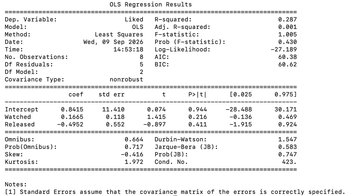
Boom. New table, new data.
And we have new coefficients, so we get:
Liked = Watched * 0.1665 + Released * -0.4952 - 0.8415
Pop that into Python with, say, our current 2026 numbers as a prediction, plus a few other ones for testing...
def Predict_Liked(Watched,Released):
 return(0.1665 * Watched + -0.4952 * Released - 0.8415)
print(Predict_Liked(89,15))
print(Predict_Liked(20,10))
print(Predict_Liked(1000,50))
And I get
6.549
-2.4635
140.8985
6.549 can be rounded up to 7, which is my current liked films seen in 2026, so that's interesting, but what about the P-values?
The P-value for Watched is 0.216 and 0.411 for Released. Both of those are over 0.05, so yeah, we can't really say that both of them have a relationship with Liked.
With R-Squared, it'll always increase if we add more variables, because we're adding more data points. So we have to look at the Adjusted R-Squared value, which is 0.001. And that is...very close to 0. So, again, no, there's no real connection.
Dangit. I guess it's just up to chance.
But hey – I finished the Data Science course!
If I felt like spending $95, I could take an exam to prove it, but...nah. I'll spend that money going to see more movies.
Day 8 — Results
- Dumbass, you can run Python on your Mac. You have it installed. You can literally just go
python movies.pyand it will do it all for you. - When you run
.ols(), you do.ols('Dependent Variable ~ Explanatory Variable', data = your_date_name). - Once you run
.ols(), you can see your coefficient for the explanatory variable and the Intercept point. Both are undercoefin the OLS table. - You can then treat that like a formula.
Dependent Variable = Explanatory-Variable-Coefficient * Explanatory Variable + Intercept. - The "P-value" is the number that tells you if there really is a relationship between the two variables.
- It's in the Coefficients data under
P>|t|. - If it's 0, there's no relationship between the variables. If it's less than 0.05, there's a pretty good chance there's a relationship between the variables. If it's over 0.05, it's unlikely there's a relationship.
- The R-Squared and Adjusted R-Squared values tell you how well the linear regression model fits your data points.
- The higher the R-Squared value, the more your data fits the function line.
- If you want to check your Dependent Variable against more Explanatory Variables in the same OLS table, it's
ols(Dependent Variable ~ Explanatory Variable 1 + Explanatory Variable 2, data = your_data_name). - Your formula is then
Dependent Variable = Explanatory Variable 1 * Explanatory Variable 1 Coefficient + Explanatory Variable 2 * Explanatory Variable 2 Coefficient - Intercept. - Because the R-Squared value keeps getting higher as you add more data points, you want to use the Adjusted R-Squared value for when you have more than one Explanatory Variable.
What am I gonna do next? I'm not sure. There's more Python. Or there's Cybersecurity, that might be funny. I suppose I'll figure out next week, since I think tomorrow and Friday will just be watching old episodes of Highlander and knitting slippers (it's gotten cold how can it get cold my feet are cold now I hate the cold).
Today's Sticker

Data Science, surrender now or prepare to fight.
MEOWTH, THAT'S RIGHT!
I don't remember where I got Meowth. Maybe it's the Shifty Thrifting Sticker Club, maybe it's Kawaii Pen Shop, maybe it's that collection I picked up from Wish ages ago. Nevertheless, Meowth is here to tell youse guys that I finished Data Science.
(I love how I don't play the card game, I don't really play the video games, but I keep putting Indigo League on TV to watch because it's just ridiculous and delightful.)