Learning Statistics, Day 5 – Fun with Averages
Guess who got a 74% average on their "Disruptive Technologies in the Digital Economy" coursework?
Guess who passed and no longer has to ever think about NFTs again unless she decides to write her dissertation on shitty digital scams?
YEAH THAT'S RIGHT, THIS DWEEB RIGHT HERE.
Well, that's a relief.
...
Back to Statistics!
Averages
The average is where most of the values are located. We saw this on Wednesday with the box-and-whiskers plot I did for my films.
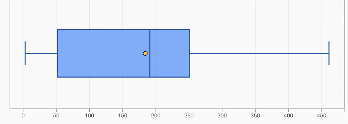
The box? That's where my averages are.
Averages are also referred to as "measures of central tendency", which seems like a lot of words for the exact same thing, but, as I learned while writing my literature review, academia sure likes using 10 words when one would do.
There are apparently different types of averages, with the most common being Mean, Median, and Mode.
Mean
The mean is what's commonly referred to as "the average". It's when you add up all the numbers, then divide that by the number of numbers.
So with my film data, you go:
3 + 8 + 29 + 74 + 157 + 191 + 205 + 245 + 257 + 394 + 461 = 2024
2024 / 11 = 184
My Mean is 184 films. I could say that, on average, I watch 184 films from each decade.
W3Schools goes into how you write out the formulas with all the fancy symbols, but I don't think I really need to know that to calculate the Mean for the population is
𝛍 = ∑𝑥₁ / 𝑛
I mean, it looks neat, but I had to spend a lot of time looking up all the special characters.
On the other hand, they also show you how to do it in NumPy using .mean()
import numpy

values = [3,8,29,74,157,191,205,245,257,394,461]

x = numpy.mean(values)

print(x)
And boom. 184. Just like all the arithmetic I did before.
They also show you how to do it in R, which is even smaller code and uses mean().
values <- c(3,8,29,74,157,191,205,245,257,394,461)

mean(values)
Which returns 184 as well. Nice.
Median
The Median is the middle value of all the data. You order all the values from smallest to largest and pick the one in the middle.
So because I have 11 values, and they're all in order anyway, this is easy. I just pick the sixth value.
3 8 29 74 157 191 205 245 257 394 461
191 is my Median.
Median isn't as affected by extreme values as much as the Mean is. If, say, I watched 1000 films from the 2010s instead of 461, my Mean would jump up to 233. But my Median would still be 191.
The formula for this is:
𝑛 + 1 / 2
Or, basically, the number of values, plus 1, divided by 2.
11 + 1 = 12
12 / 2 = 6
The sixth value. 191.
When you have an odd number of values, like I do, it's a whole number. But when it's an even number, it's between the two observations.
So if we take off the 461 from my list, we have
3 8 29 74 157 191 205 245 257 394
And that'd be the 5.5th value. So the Median in this case would be the Mean of the values on either side of that point, which are 157 and 191.
So I do the maths...
157 + 191 = 348
348 / 2 = 174
And 174 is my Median.
Luckily, NumPy has .median() to make my life so much easier.
import numpy

values = [3,8,29,74,157,191,205,245,257,394,461]

x = numpy.median(values)

print(x)
And there's our 191.
If I do the even-number value set...
import numpy

values = [3,8,29,74,157,191,205,245,257,394]

x = numpy.median(values)

print(x)
And there's our 174 without me having to individually count each value.
R has the median() function, which is so much smaller and neater.
values <- c(3,8,29,74,157,191,205,245,257,394,461)

median(values)
(You know, I'm thinking that if I'm going to be doing more statistics in the future, I might want to look at R. It does seem to be awfully nice.)
For Median, it helps if your data is already ordered from smallest to highest, but having just tested moving around the numbers in NumPy, I don't think it makes that much of a difference when you're programming it in. Like, I just moved around the numbers and it's still giving me the same results. Which is nice, especially when you're thinking about bigger data sets.
Mode
Mode is the value that appears the most often in the data. Since my decades film data doesn't have duplicates, I'm going to use my 2010-2019 year data.
43 51 42 50 44 41 49 53 41 47
41 shows up twice in that list, so 41 is my Mode.
You can also use Mode for categorial data. So if I take the 15 films I've seen that were released in 2026 and list their genres:
Science Fiction, Action, Adventure
Animation, Action, Fantasy, Adventure
Adventure, Action, Fantasy
Science Fiction, Action, Adventure
Horror, Comedy, Romance
Mystery, Science Fiction, Horror
Thriller, Action, Comedy
Horror, Action, Thriller
Comedy, Horror
Comedy, Science Fiction, Adventure
Crime, Drama
Horror, Science Fiction, Fantasy
Comedy
Thriller, Horror, Comedy
Horror, Science Fiction, Thriller
Horror is my Mode, because that has 7 films listed under that genre.
(Oh, and if you're wondering, those 15 are:
- Spider-Man: Brand New Day
- Avatar Aang: The Last Airbender
- The Odyssey
- The Mandalorian and Grogu
- Teenage Sex and Death at Camp Miasma
- Backrooms
- Over Your Dead Body
- Pretty Lethal
- Ready or Not 2: Here I Come
- Project Hail Mary
- Peaky Blinders: The Immortal Man
- The Bride
- I Want Your Sex
- Send Help
- 28 Years Later: The Bone Temple )
Because there's only one value that shows up multiple times, that's a Unimodal distribution.
But you can have multiple Modes, as long as they all appear the same number of times in the data. So if I take Horror out, then my Mode is Action, Comedy, Science Fiction. This is Multimodal distribution. If there were only two Modes, it'd be Bimodal distribution.
In Python, you import in the Statistics library and use multimode.
To get the Mode in a numerical list:
from statistics import multimode

values = [43,51,42,50,44,41,49,53,41,47]

x = multimode(values)

print(x)
That gets me my 41 without me having to organise the data.
R is a little more complicated this time, because it doesn't have a built-in function to find the mode.
mode <- function(x) {
    unique_values <- unique(x)
    table <- tabulate(match(x, unique_values))
    unique_values[table == max(table)]
}

values <- c(43,51,42,50,44,41,49,53,41,47)

mode(values)
But I still get my 41.
There must be a way to get a Mode for a categorical list in Python, but they don't mention it, and trying to put the categorical list into the Python used for the numerical list just brings up an error. But I'm sure something exists – I just have to find it.
Day 5 — Results
- Averages are where most of the values in your data are located.
- They're also known as measures of central tendency.
- The most common averages are Mean, Median, and Mode.
- Mean is when you add up all your numerical data and then divide that by the number of rows in your data.
- You can find it in NumPy by using
.mean()or in R by usingmean(). - Median is the middle value of your numerical data if it's sorted smallest to largest.
- When you have an odd number of data rows, Median is the value right in the middle.
- When you have an even number of data rows, Median is the Mean of the two values where your Median would be.
- You can find it in NumPy using
.median()or in R by usingmedian(). - Mode is the value that appears the most in the data.
- You can use Mode on numerical and categorical data.
- Data with one Mode is called a Unimodal distribution.
- Data with two Modes is called Bimodal distribution.
- Data with multiple Modes is Multimodal distribution.
- You can find the Mode in your numerical data in Python by using the Statistics library and using
multimode. - You can't use
multimodeto find the Mode in your categorical data. - There also isn't a built-in function in R to find the Mode.
I thought about going further and doing everything on Variation, but I think that this is enough mathematics for my brain today.
No, now it's time for Valheim and Highlander. Good.
Today's Sticker

Bandit looks like he's having a midlife crisis.
Oh Bandit, I've been there. Have I ever been there.